As GSoC 2025 comes to an end, here is my final working outcome of the project. I’ve showed this with a help of a real world use case. In this case study we’ll compare two techniques for cooling batteries in EVs and will draw out a conclusion which is better.
Context of project:
For my Google Summer of Code project, I’ve added a cool new feature to PyBaMM. My goal is to let it run 3D thermal simulations that work together with its battery models. This will help us understand how batteries heat up in 3D.
Work So Far:
Before beginning the case study, here are all my PRs I worked on:
- 3D FEM: Added 3D Submeshes and 3D Finite Element Method.
- 3D Thermal Model: Added
Basic3DThermalSPMmodel with two way coupling. - 2D & 3D Heatmaps: Added
plot_3d_cross_section&plot_3d_heatmap functionsto support plotting for 3D thermal simulation.
Apart from this I patched up few non-deterministic bugs in PyBaMM:
- Shape Error in 3D FEM
- Non deterministic CI issues in Plotting
- Few more fixes for non-deterministic issues
After this all CI issues were patched up, I also started working on a stretch goal to improve the existing mesh functionality:
- Added
load_mesh_from_filefunction to support external 3D meshes: Added helper functions to import external 3D meshes generated from other tools or libraries which can be solved in PyBaMM. This can help users get high quality meshes from other libraries which we can’t directly support in PyBaMM due to licensing issues.
Case Study: Comparing Thermal Management Strategies for a Cylindrical EV Battery
You can directly copy paste the code and try running this, all 3D functionality is now available in PyBaMM!
1. Motivation
Effective thermal management is critical for the safety, performance, and lifespan of lithium-ion batteries in electric vehicles (EVs). Engineers must often choose between different cooling strategies, each with its own trade-offs.
This notebook simulates and compares two common cooling strategies for a cylindrical cell under a high-power discharge:
- Uniform Air Cooling: A baseline strategy where the cell is cooled evenly on all surfaces by airflow. This is simpler and cheaper to implement.
- Base Cooling: An engineered strategy where the cell is mounted on a liquid-cooled plate, providing strong cooling to the base while the other surfaces are exposed to air.
2. Running the Simulations
We will run two separate simulations, one for each cooling strategy. All electrochemical parameters and the discharge profile (2C) will be kept identical to ensure a fair comparison.
ln[1]:
import matplotlib.pyplot as plt
import numpy as np
from matplotlib.widgets import Slider
from scipy.interpolate import griddata

import pybamm

%pip install ipympl
%matplotlib widget
ln[2]:
# --- Define the two cooling strategies ---
cooling_strategies = {
    "Uniform Air Cooling": {
        "Outer radius heat transfer coefficient [W.m-2.K-1]": 5,  # Passive air cooling
        "Inner radius heat transfer coefficient [W.m-2.K-1]": 5,
        "Top face heat transfer coefficient [W.m-2.K-1]": 5,
        "Bottom face heat transfer coefficient [W.m-2.K-1]": 5,
    },
    "Base Cooling": {
        "Outer radius heat transfer coefficient [W.m-2.K-1]": 10,
        "Inner radius heat transfer coefficient [W.m-2.K-1]": 10,
        "Top face heat transfer coefficient [W.m-2.K-1]": 10,
        "Bottom face heat transfer coefficient [W.m-2.K-1]": 200,  # Strong base cooling
    },
}

solutions = {}
print("--- Running Simulations for Each Cooling Strategy ---")

for name, params in cooling_strategies.items():
    print(f"\nSolving for: {name}...")
    model_3d = pybamm.lithium_ion.Basic3DThermalSPM(
        options={"cell geometry": "cylindrical", "dimensionality": 3}
    )
    parameter_values = pybamm.ParameterValues("Chen2020")
    parameter_values.update(
        {
            "Inner cell radius [m]": 0.005,
            "Outer cell radius [m]": 0.018,
            "Cell height [m]": 0.065,
        },
        check_already_exists=False,
    )
    parameter_values.update(params, check_already_exists=False)

    experiment = pybamm.Experiment(["Discharge at 2C until 2.8 V"])
    var_pts = {
        "x_n": 25,
        "x_s": 25,
        "x_p": 25,
        "r_n": 35,
        "r_p": 35,
        "z": None,
        "r_macro": None,
    }
    submesh_types = model_3d.default_submesh_types
    submesh_types["cell"] = pybamm.ScikitFemGenerator3D(
        "cylinder", h="0.01"
    )  # fine mesh

    sim = pybamm.Simulation(
        model_3d,
        parameter_values=parameter_values,
        var_pts=var_pts,
        experiment=experiment,
    )
    solutions[name] = sim.solve()
    print(f"'{name}' simulation complete.")
3. Interactive Dashboards
Now we will generate the interactive dashboards for each cooling strategy to explore the results.
ln[3]:
# --- Define the Common AnimationUpdater Class Once ---
# This class contains all the logic for updating the interactive plots.
class AnimationUpdater:
    def __init__(self, fig, solution, axes_dict, cax_3d):
        self.fig = fig
        self.solution = solution
        self.axes = axes_dict
        self.cax_3d = cax_3d

        self.times = self.solution.t
        self.voltages = self.solution["Voltage [V]"].data
        self.avg_temps_c = (
            self.solution["Volume-averaged cell temperature [K]"].data - 273.15
        )
        self.temp_func = self.solution["Cell temperature [K]"]
        self.mesh = self.temp_func.mesh
        self.nodes = self.mesh.nodes
        self.x_nodes, self.y_nodes, self.z_nodes = (
            self.nodes[:, 0],
            self.nodes[:, 1],
            self.nodes[:, 2],
        )
        self.r_nodes = np.sqrt(self.x_nodes**2 + self.y_nodes**2)

        all_temps_k = self.solution["Cell temperature [K]"].entries
        self.global_min_temp = np.min(all_temps_k) - 273.15
        self.global_max_temp = np.max(all_temps_k) - 273.15
        self.levels = np.linspace(self.global_min_temp, self.global_max_temp, 25)

        self.cb_xy, self.cb_rz = None, None

        self.axes["voltage"].plot(self.times, self.voltages, "b-")
        (self.voltage_marker,) = self.axes["voltage"].plot([], [], "ro")
        self.axes["voltage"].set_title("Terminal Voltage")
        self.axes["voltage"].set_xlabel("Time [s]")
        self.axes["voltage"].set_ylabel("Voltage [V]")
        self.axes["voltage"].grid(True, alpha=0.3)

        self.axes["avg_temp"].plot(self.times, self.avg_temps_c, "r-")
        (self.temp_marker,) = self.axes["avg_temp"].plot([], [], "bo")
        self.axes["avg_temp"].set_title("Average Cell Temperature")
        self.axes["avg_temp"].set_xlabel("Time [s]")
        self.axes["avg_temp"].set_ylabel("Temperature [°C]")
        self.axes["avg_temp"].grid(True, alpha=0.3)

        self.setup_interpolation_grids()
        self.update_plots(self.times[0])

    def setup_interpolation_grids(self):
        r_min, r_max = self.r_nodes.min(), self.r_nodes.max()
        z_min, z_max = self.z_nodes.min(), self.z_nodes.max()
        self.r_grid_polar = np.linspace(r_min, r_max, 60)
        self.theta_grid_polar = np.linspace(0, 2 * np.pi, 60)
        self.R_grid_polar, self.Theta_grid_polar = np.meshgrid(
            self.r_grid_polar, self.theta_grid_polar
        )
        self.r_grid_rz = np.linspace(r_min, r_max, 60)
        self.z_grid_rz = np.linspace(z_min, z_max, 60)
        self.R_grid_rz, self.Z_grid_rz = np.meshgrid(self.r_grid_rz, self.z_grid_rz)

    def update_plots(self, current_time):
        current_voltage = np.interp(current_time, self.times, self.voltages)
        current_avg_temp = np.interp(current_time, self.times, self.avg_temps_c)
        self.voltage_marker.set_data([current_time], [current_voltage])
        self.temp_marker.set_data([current_time], [current_avg_temp])

        ax_xy, ax_rz, ax_3d = self.axes["xy"], self.axes["rz"], self.axes["3d"]
        if self.cb_xy:
            self.cb_xy.remove()
        if self.cb_rz:
            self.cb_rz.remove()
        ax_xy.clear()
        ax_3d.clear()
        ax_rz.clear()

        temp_nodes_c = (
            self.temp_func(
                t=current_time, x=self.x_nodes, y=self.y_nodes, z=self.z_nodes
            )
            - 273.15
        )

        z_mid = (self.z_nodes.min() + self.z_nodes.max()) / 2
        xy_mask = (
            np.abs(self.z_nodes - z_mid)
            < (self.z_nodes.max() - self.z_nodes.min()) * 0.3
        )
        if np.sum(xy_mask) > 10:
            r_xy, theta_xy, temp_xy = (
                self.r_nodes[xy_mask],
                np.arctan2(self.y_nodes[xy_mask], self.x_nodes[xy_mask]),
                temp_nodes_c[xy_mask],
            )
            grid_points = np.column_stack(
                [self.R_grid_polar.ravel(), self.Theta_grid_polar.ravel()]
            )
            temp_interp_xy = griddata(
                np.column_stack([r_xy, theta_xy]),
                temp_xy,
                grid_points,
                method="linear",
                fill_value=np.nan,
            )
            if np.any(np.isnan(temp_interp_xy)):
                temp_interp_xy[np.isnan(temp_interp_xy)] = griddata(
                    np.column_stack([r_xy, theta_xy]),
                    temp_xy,
                    grid_points[np.isnan(temp_interp_xy)],
                    method="nearest",
                )
            temp_interp_xy = temp_interp_xy.reshape(self.R_grid_polar.shape)
            cont_xy = ax_xy.contourf(
                self.Theta_grid_polar,
                self.R_grid_polar,
                temp_interp_xy,
                levels=self.levels,
                cmap="coolwarm",
                extend="both",
            )
            ax_xy.set_title(f"XY Cross-section (z≈{z_mid * 1000:.1f}mm)")
            ax_xy.grid(True, alpha=0.3)
            self.cb_xy = self.fig.colorbar(cont_xy, ax=ax_xy, label="Temperature [°C]")

        rz_mask = np.abs(self.y_nodes) < max(
            0.001, (self.y_nodes.max() - self.y_nodes.min()) * 0.2
        )
        if np.sum(rz_mask) > 10:
            r_rz, z_rz, temp_rz = (
                self.r_nodes[rz_mask],
                self.z_nodes[rz_mask],
                temp_nodes_c[rz_mask],
            )
            grid_points_rz = np.column_stack(
                [self.R_grid_rz.ravel(), self.Z_grid_rz.ravel()]
            )
            temp_interp_rz = griddata(
                np.column_stack([r_rz, z_rz]),
                temp_rz,
                grid_points_rz,
                method="linear",
                fill_value=np.nan,
            )
            if np.any(np.isnan(temp_interp_rz)):
                temp_interp_rz[np.isnan(temp_interp_rz)] = griddata(
                    np.column_stack([r_rz, z_rz]),
                    temp_rz,
                    grid_points_rz[np.isnan(temp_interp_rz)],
                    method="nearest",
                )
            temp_interp_rz = temp_interp_rz.reshape(self.R_grid_rz.shape)
            cont_rz = ax_rz.contourf(
                self.R_grid_rz * 1000,
                self.Z_grid_rz * 1000,
                temp_interp_rz,
                levels=self.levels,
                cmap="coolwarm",
                extend="both",
            )
            ax_rz.set_title("RZ Cross-section: Gradient")
            ax_rz.set_xlabel("Radius [mm]")
            ax_rz.set_ylabel("Height [mm]")
            ax_rz.set_aspect("equal", "box")
            ax_rz.grid(True, alpha=0.3)
            self.cb_rz = self.fig.colorbar(cont_rz, ax=ax_rz, label="Temperature [°C]")

        scatter = ax_3d.scatter(
            self.x_nodes * 1000,
            self.y_nodes * 1000,
            self.z_nodes * 1000,
            s=25,
            c=temp_nodes_c,
            cmap="coolwarm",
            vmin=self.global_min_temp,
            vmax=self.global_max_temp,
            alpha=0.7,
        )
        ax_3d.set_title(f"3D Heatmap ({len(self.nodes)} nodes)")
        ax_3d.set_xlabel("x [mm]")
        ax_3d.set_ylabel("y [mm]")
        ax_3d.set_zlabel("z [mm]")
        ax_3d.view_init(elev=25, azim=-60)
        self.fig.colorbar(scatter, cax=self.cax_3d, label="Temperature [°C]")

        self.fig.suptitle(
            f"3D Thermal Battery Model - Time: {current_time:.1f}s, Voltage: {current_voltage:.2f}V, Avg Temp: {current_avg_temp:.2f}°C",
            fontsize=16,
        )
        self.fig.canvas.draw_idle()
Uniform Cooling
ln[5]:
fig1 = plt.figure(figsize=(14, 7))
fig1.suptitle("Uniform Air Cooling Simulation", fontsize=18, fontweight="bold")
gs1 = fig1.add_gridspec(2, 4, width_ratios=(1.5, 1, 1, 0.1), height_ratios=(1, 1))

plt.subplots_adjust(
    left=0.05, right=0.92, bottom=0.15, top=0.85, hspace=0.5, wspace=0.5
)

axes1 = {
    "voltage": fig1.add_subplot(gs1[0, 0]),
    "avg_temp": fig1.add_subplot(gs1[1, 0]),
    "xy": fig1.add_subplot(gs1[0, 1], projection="polar"),
    "3d": fig1.add_subplot(gs1[0, 2], projection="3d"),
    "rz": fig1.add_subplot(gs1[1, 1]),
}
cax_3d_1 = fig1.add_subplot(gs1[0, 3])

slider_ax1 = plt.axes([0.25, 0.05, 0.5, 0.03])
time_slider1 = Slider(
    slider_ax1,
    "Time (s)",
    solutions["Uniform Air Cooling"].t[0],
    solutions["Uniform Air Cooling"].t[-1],
    valinit=0,
)

updater1 = AnimationUpdater(fig1, solutions["Uniform Air Cooling"], axes1, cax_3d_1)
time_slider1.on_changed(updater1.update_plots)

plt.show()
 (open in new tab for gif animation)
Base Cooling
ln[6]:
fig2 = plt.figure(figsize=(14, 7))
fig2.suptitle("Base Cooling Simulation", fontsize=18, fontweight="bold")
gs2 = fig2.add_gridspec(2, 4, width_ratios=(1.5, 1, 1, 0.1), height_ratios=(1, 1))

plt.subplots_adjust(
    left=0.05, right=0.92, bottom=0.15, top=0.85, hspace=0.5, wspace=0.5
)

axes2 = {
    "voltage": fig2.add_subplot(gs2[0, 0]),
    "avg_temp": fig2.add_subplot(gs2[1, 0]),
    "xy": fig2.add_subplot(gs2[0, 1], projection="polar"),
    "3d": fig2.add_subplot(gs2[0, 2], projection="3d"),
    "rz": fig2.add_subplot(gs2[1, 1]),
}
cax_3d_2 = fig2.add_subplot(gs2[0, 3])

slider_ax2 = plt.axes([0.25, 0.05, 0.5, 0.03])
time_slider2 = Slider(
    slider_ax2,
    "Time (s)",
    solutions["Base Cooling"].t[0],
    solutions["Base Cooling"].t[-1],
    valinit=0,
)

updater2 = AnimationUpdater(fig2, solutions["Base Cooling"], axes2, cax_3d_2)
time_slider2.on_changed(updater2.update_plots)

plt.show()
 (open in new tab for gif animation)
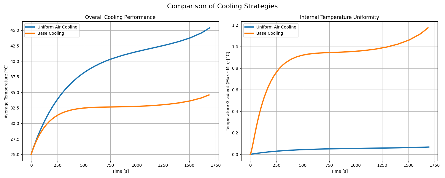
4. Comparative Analysis
This plot provides the key summary of the results. It directly compares the main performance metrics for both cooling strategies, telling the story of the engineering trade-offs.
5. Conclusion
The comparative analysis clearly shows the engineering trade-offs between the two cooling strategies:
- Uniform Air Cooling is less effective at removing heat, leading to a higher overall average temperature. However, it results in a very uniform internal temperature, minimizing the gradient across the cell.
- Base Cooling is much more effective, keeping the average cell temperature significantly lower. The drawback is the creation of a large internal temperature gradient, which can accelerate localized degradation and aging if not managed properly.
This case study demonstrates how 3D thermal modeling is a crucial tool for engineers to understand and optimize battery pack design for safety and longevity.
Final Thoughts
This GSoC 2025 was an amazing experience, thanks to all my mentors for being so cool and guiding me throughout this project. I am really enjoying the overall open source experience!